import numpy as np
import pandas as pd
import matplotlib.pyplot as plt
import seaborn as sns
from sklearn.cluster import KMeansClustering of Shopping Data with K-means Clustering
Clustering
K-means
In this blog post, our primary focus will be on exploring a machine-learning project centered on the creation of customer clusters through K-means clustering. The process starts with gaining a thorough understanding of the dataset, followed by visualizing key features and processing the data. The dataset includes information such as gender, age, annual income, and spending score. Moving forward, we will undertake the task of training and evaluating a K-means clustering model to generate clusters based on this dataset.
Importing Libraries
In this section, essential libraries are imported for various tasks. NumPy and Pandas are utilized for data manipulation, while Matplotlib.pyplot and Seaborn are employed for data visualization. Additionally, the KMeans module from sklearn.cluster is imported for implementing the clustering algorithm.
Exploring Dataset and Visualization
In this segment, the dataset is explored first. In this code snippet, the pd.read_csv() function is employed to load the dataset named ‘Mall_Customers.csv’ into a pandas DataFrame, designated as mall_data. Subsequently, the head() and info() functions are utilized to provide a rapid overview of the dataset, displaying the initial rows and essential information such as data types and missing values.
mall_data = pd.read_csv("Mall_Customers.csv")
mall_data.head()
mall_data.info()
<class 'pandas.core.frame.DataFrame'>
RangeIndex: 200 entries, 0 to 199
Data columns (total 5 columns):
# Column Non-Null Count Dtype
--- ------ -------------- -----
0 CustomerID 200 non-null int64
1 Gender 200 non-null object
2 Age 200 non-null int64
3 Annual Income (k$) 200 non-null int64
4 Spending Score (1-100) 200 non-null int64
dtypes: int64(4), object(1)
memory usage: 7.9+ KBmall_data.info()<class 'pandas.core.frame.DataFrame'>
RangeIndex: 200 entries, 0 to 199
Data columns (total 5 columns):
# Column Non-Null Count Dtype
--- ------ -------------- -----
0 CustomerID 200 non-null int64
1 Gender 200 non-null object
2 Age 200 non-null int64
3 Annual Income (k$) 200 non-null int64
4 Spending Score (1-100) 200 non-null int64
dtypes: int64(4), object(1)
memory usage: 7.9+ KBIn this section, the correlation matrix of the dataset is computed using the corr() function, and the results are visualized through a heatmap generated with the Seaborn library.
# Exclude non-numeric columns before computing correlation
numeric_columns = mall_data.select_dtypes(include=[np.number])
corr = numeric_columns.corr()

# Visualization of correlation matrix
plt.figure(figsize=(8, 8))
sns.heatmap(corr, cbar=True, square=True, fmt='.1f', annot=True, cmap='Reds')
<Axes: >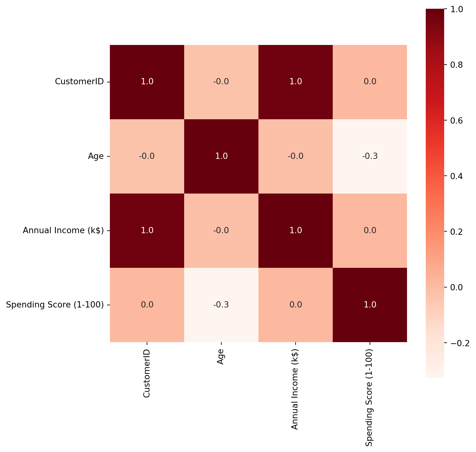
In this segment, multiple plots are generated to visually represent the data distribution and relationships among various features. This includes count plots for ‘Gender’ and ‘Age’, as well as a bar plot illustrating the relationship between ‘Annual Income’ and ‘Spending Score’.
plt.figure(figsize=(10,10))
sns.countplot(x="Gender", data=mall_data)
<Axes: xlabel='Gender', ylabel='count'>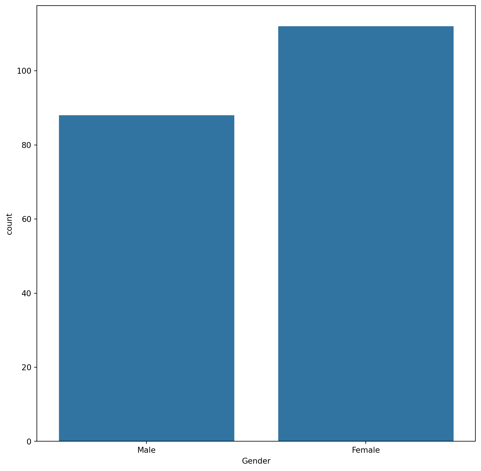
plt.figure(figsize=(16,10))
sns.countplot(x="Age", data=mall_data)
<Axes: xlabel='Age', ylabel='count'>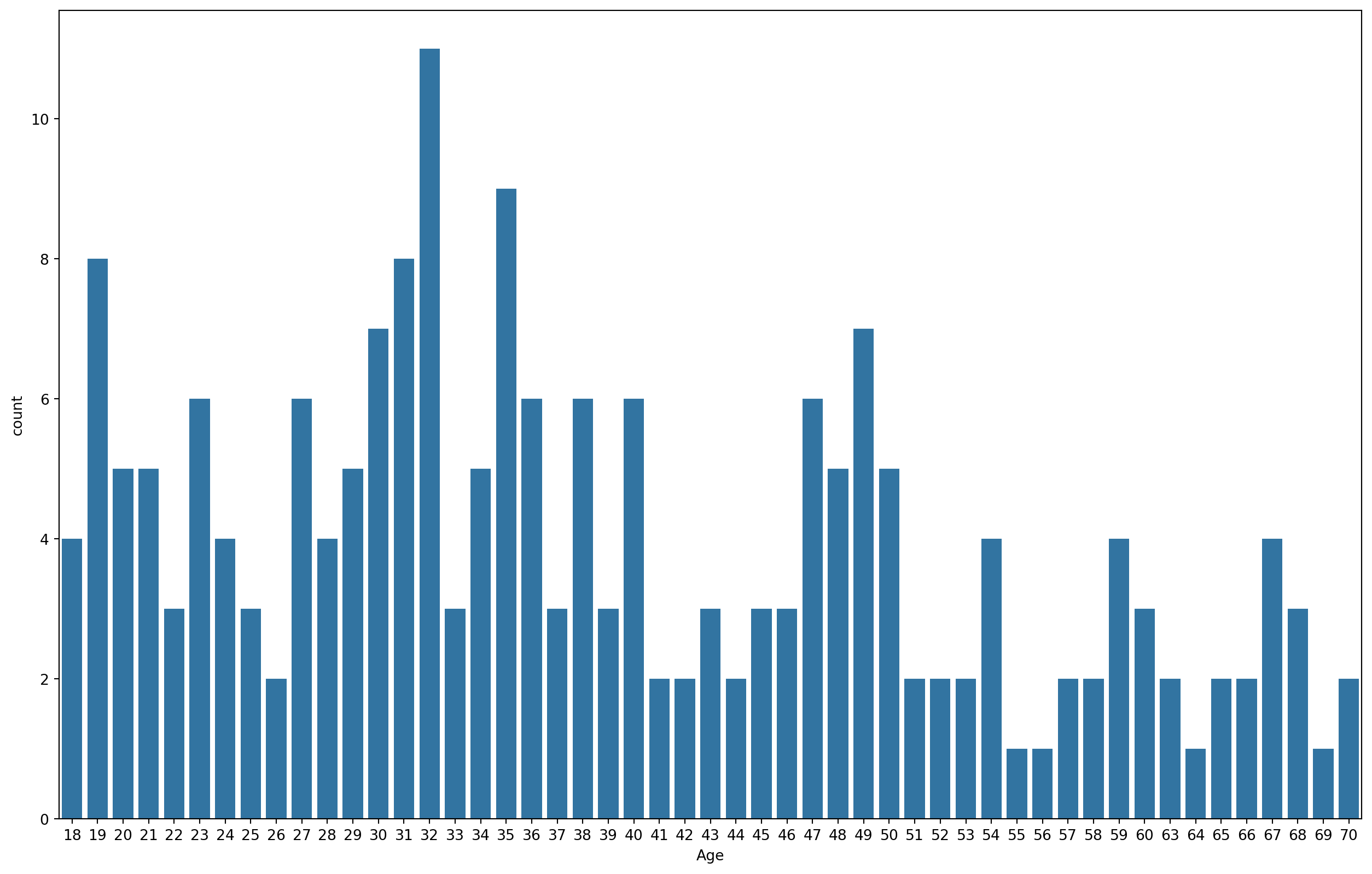
plt.figure(figsize=(20,8))
sns.barplot(x='Annual Income (k$)',y='Spending Score (1-100)',data=mall_data)
<Axes: xlabel='Annual Income (k$)', ylabel='Spending Score (1-100)'>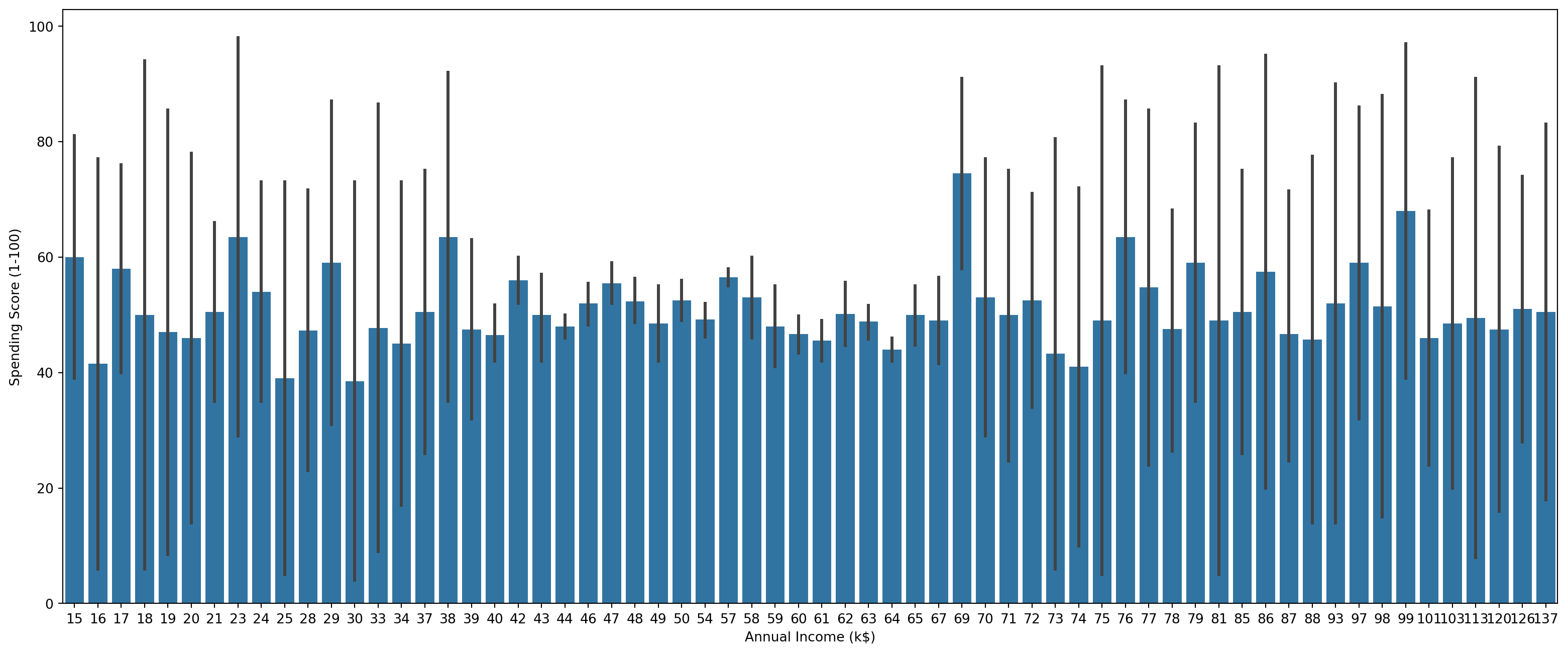
Clusters
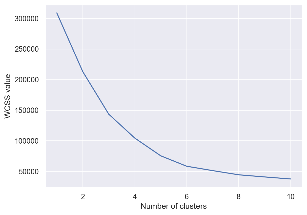
This section prepares the data for clustering and determines the optimal number of clusters using the Elbow Method. The iloc function is used to select specific columns from the DataFrame to create a new variable X, which will be used for clustering. The code then fits the K-Means algorithm to the data for a range of cluster numbers (from 1 to 10) and calculates the Within-Cluster-Sum-of-Squares (WCSS). Then, a plot is created to visualize the Within-Cluster Sum of Squares (WCSS) against the number of clusters. This plot is instrumental in identifying the ‘elbow,’ aiding in the determination of the optimal number of clusters for the dataset.
X = mall_data.iloc[:,[2,3,4]].values
wcss = []
for i in range(1,11): # It will find wcss value for different number of clusters (for 1 cluster, for 2...until 10 clusters) and put it in our list
    kmeans = KMeans(n_clusters=i, init='k-means++', random_state=50)
    kmeans.fit(X)
    wcss.append(kmeans.inertia_)
sns.set()
plt.plot(range(1,11),wcss)
plt.xlabel("Number of clusters")
plt.ylabel("WCSS value")
plt.show()
C:\Users\USER\AppData\Local\Packages\PythonSoftwareFoundation.Python.3.9_qbz5n2kfra8p0\LocalCache\local-packages\Python39\site-packages\sklearn\cluster\_kmeans.py:1416: FutureWarning:
The default value of `n_init` will change from 10 to 'auto' in 1.4. Set the value of `n_init` explicitly to suppress the warning
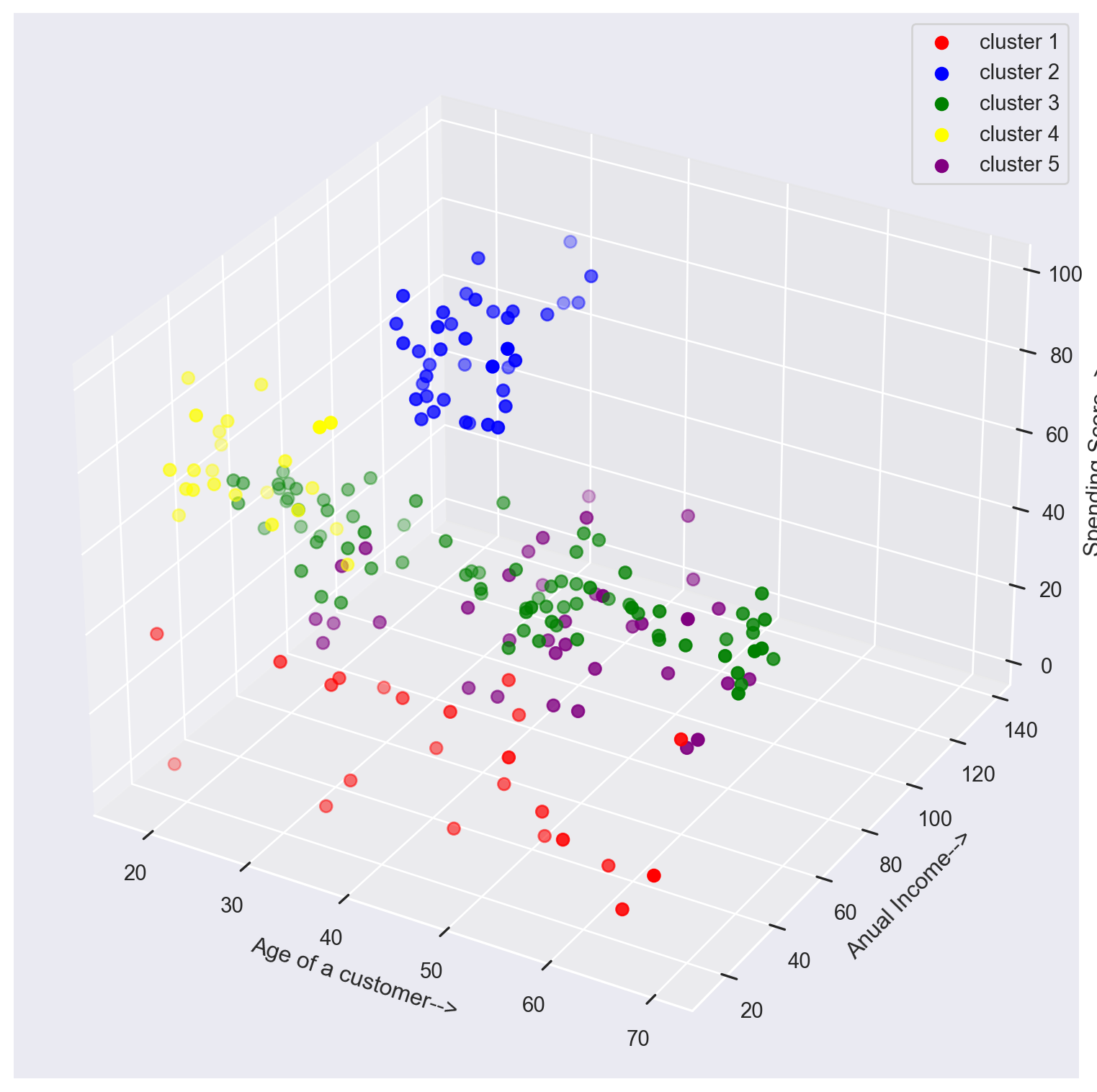
In this step, the K-Means algorithm is applied to the data using the optimal number of clusters determined in the previous step. The fit_predict() function is employed to calculate cluster centers and predict the cluster index for each sample in the dataset. And then the clusters are visualized.
kmeans = KMeans(n_clusters = 5, init = 'k-means++',random_state = 0)
y = kmeans.fit_predict(X)
fig = plt.figure(figsize = (10,10))
ax = fig.add_subplot(111, projection='3d')
ax.scatter(X[y == 0,0],X[y == 0,1],X[y == 0,2], s = 40 , color = 'red', label = "cluster 1")
ax.scatter(X[y == 1,0],X[y == 1,1],X[y == 1,2], s = 40 , color = 'blue', label = "cluster 2")
ax.scatter(X[y == 2,0],X[y == 2,1],X[y == 2,2], s = 40 , color = 'green', label = "cluster 3")
ax.scatter(X[y == 3,0],X[y == 3,1],X[y == 3,2], s = 40 , color = 'yellow', label = "cluster 4")
ax.scatter(X[y == 4,0],X[y == 4,1],X[y == 4,2], s = 40 , color = 'purple', label = "cluster 5")
ax.set_xlabel('Age of a customer-->')
ax.set_ylabel('Anual Income-->')
ax.set_zlabel('Spending Score-->')
ax.legend()
plt.show()
C:\Users\USER\AppData\Local\Packages\PythonSoftwareFoundation.Python.3.9_qbz5n2kfra8p0\LocalCache\local-packages\Python39\site-packages\sklearn\cluster\_kmeans.py:1416: FutureWarning:
The default value of `n_init` will change from 10 to 'auto' in 1.4. Set the value of `n_init` explicitly to suppress the warning
Conclusion
As observed, clusters 3 and 5 exhibit higher spending scores.
For Cluster 3, comprising individuals aged less than 30 with very high annual incomes, their elevated spending scores align with expectations. To sustain and enhance this trend, offering these individuals improved incentives and exclusive deals could be an effective strategy.
Cluster 5 consists of individuals aged less than 30 with comparatively lower incomes. Despite their lower financial capacity, this group shows a preference for shopping. To further engage them, enticing offers such as discounts and additional freebies could be implemented to augment their spending within the establishment.