Netflix Stock Prediction

This blog provides a comprehensive demonstration of loading, visualizing, and analyzing time-series data in Python. It also illustrates the implementation of ARIMA predictions for stock price prediction. The script showcases how to evaluate the model’s performance and generate plots depicting the best and worst predictions.

ARIMA, or AutoRegressive Integrated Moving Average, is a time series forecasting model that combines autoregression, differencing, and moving averages to predict future values based on historical patterns, making it widely used for stock price predictions.

Importing Libraries

The script begins by importing a variety of essential libraries, each serving a specific purpose. NumPy is utilized for numerical operations, Pandas for data manipulation and analysis, Plotly for interactive plotting, Seaborn and Matplotlib for statistical data visualization, fbprophet for time series forecasting, pandas_datareader for remote data access, SciPy for scientific computing, scikit-learn (sklearn) for machine learning, and Statsmodels for statistical models. These libraries collectively provide a comprehensive set of tools for tasks ranging from data manipulation and visualization to time series forecasting, machine learning, and statistical modeling.

import random 
import numpy as np 
import pandas as pd 
import plotly.express as px
import seaborn as sns
import matplotlib.pyplot as plt
import plotly.graph_objects as go
import matplotlib.ticker as ticker
import plotly.figure_factory as ff
from statsmodels.tsa.arima.model import ARIMA  
from pandas_datareader import data
from scipy import stats
from sklearn.metrics import mean_absolute_error
from statsmodels.tsa.seasonal import seasonal_decompose
from sklearn.preprocessing import MinMaxScaler
from matplotlib.ticker import FixedFormatter, FixedLocator

Exploring Dataset and Visualization

The script begins by reading a CSV file containing Netflix’s stock prices into a Pandas DataFrame. Following this, it displays the column names of the DataFrame. Subsequently, the script creates a plot illustrating the volume of Netflix’s stock against the date. Additionally, it generates a histogram of the closing prices of Netflix’s stock, accompanied by vertical lines indicating the mean, median, and mode of the closing prices. These visualizations provide insights into the distribution and trends within the stock data.

path = "NFLX.csv"
prices_train = pd.read_csv(path)
pd.DataFrame(prices_train.columns, columns=["name"])

	name
0	Date
1	Open
2	High
3	Low
4	Close
5	Adj Close
6	Volume

fig = px.bar(prices_train, x='Date', y='Volume')
fig.update_layout(title=f'Netflix stock price', barmode='stack', font_color="black")
fig.show()

f, (ax1) = plt.subplots(1, 1, figsize=(14, 5))
v_dist_1 = prices_train["Close"].values
sns.histplot(v_dist_1, ax=ax1, kde=True)
mean=prices_train["Close"].mean()
median=prices_train["Close"].median()
mode=prices_train["Close"].mode().values[0]
ax1.axvline(mean, color='r', linestyle='--', label="Mean")
ax1.axvline(median, color='g', linestyle='-', label="Mean")
ax1.axvline(mode, color='b', linestyle='-', label="Mode")
ax1.legend()

<matplotlib.legend.Legend at 0x1a66c662220>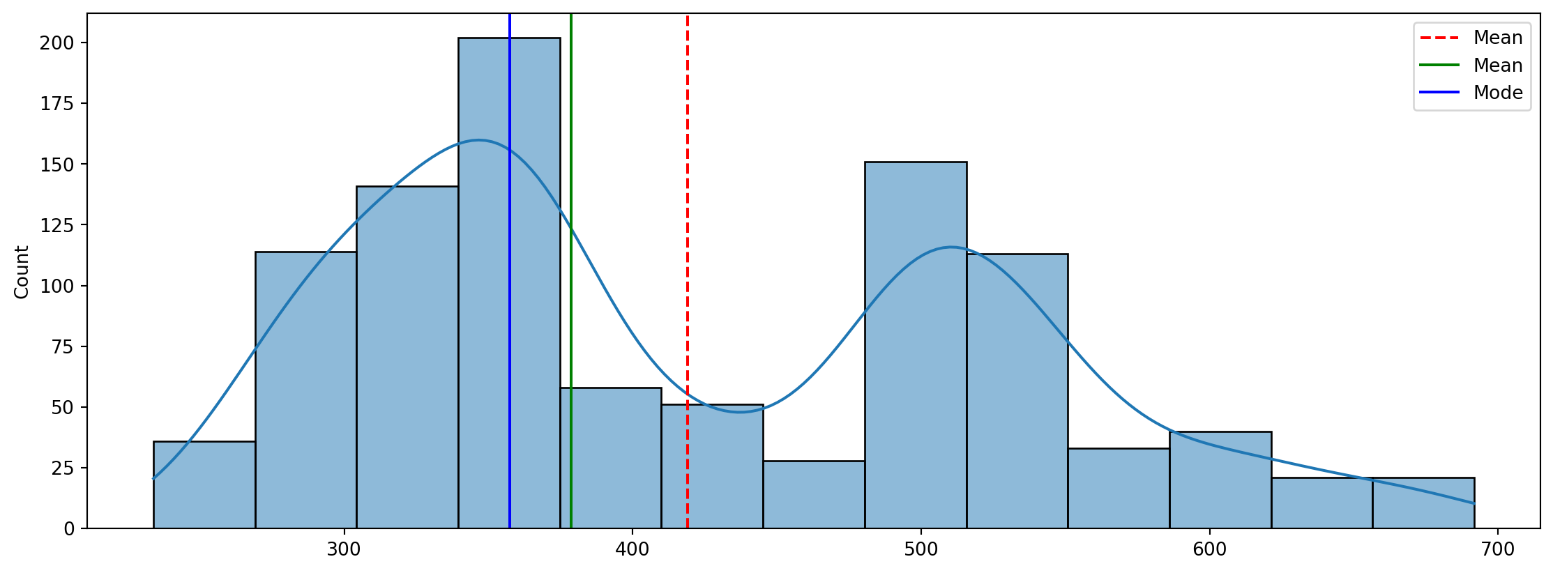

ARIMA simulation

In this section of the script, the data is prepared for ARIMA prediction. This involves calculating the daily returns of the closing prices, determining the drift (which represents the average daily return adjusted for variance), and generating random variables for the simulation. These steps are crucial where random future scenarios are generated based on historical data to estimate potential future stock prices.

days_prev_len = 20

# Use the "Close" column for stock prices
prices_train_copy = prices_train["Close"]

# Split the data into training and testing sets
train_size = int(len(prices_train_copy) * 0.8)
train = prices_train_copy[0:train_size]
test = prices_train_copy[train_size:train_size + days_prev_len]

# Example order for ARIMA (p, d, q)
order = (5, 1, 2)  # You can experiment with these parameters

# Fit ARIMA model
model = ARIMA(train, order=order)
fit_model = model.fit()

# Forecast future prices
forecast = fit_model.get_forecast(steps=len(test))
predictions = forecast.predicted_mean

C:\Users\USER\AppData\Local\Packages\PythonSoftwareFoundation.Python.3.9_qbz5n2kfra8p0\LocalCache\local-packages\Python39\site-packages\statsmodels\base\model.py:607: ConvergenceWarning:

Maximum Likelihood optimization failed to converge. Check mle_retvals

Run the prediction.

The script proceeds to execute the ARIMA prediction. It involves calculating daily returns for each day and each simulation, then determining stock prices for each day and each simulation based on these daily returns. Finally, the script plots the simulated stock prices, providing a visual representation of the potential future trajectories of Netflix’s stock based on the ARIMA Prediction.

def get_plot_simulation(predictions: pd.Series):
    fig = px.line(title='ARIMA Stock Price Prediction')
    fig.add_scatter(y=predictions, name='ARIMA Predictions')
    fig.update_layout(paper_bgcolor='white', plot_bgcolor="white", font_color="black")
    fig.show()

# Assuming 'predictions' is the Series obtained from the ARIMA model
get_plot_simulation(predictions)

Evaluate the model.

Following the prediction, the script calculates the mean absolute error of the model’s predictions on the test data for each simulation. Subsequently, it plots the prediction with the smallest error and the prediction with the largest error alongside the actual test data. This visual representation helps in assessing the model’s performance by showcasing the predictions with the best and worst accuracy in comparison to the actual test data.

# Calculate mean absolute error for ARIMA predictions
mae_arima = mean_absolute_error(test, predictions)

# Print the Mean Absolute Error for ARIMA predictions
print(f"MAE for ARIMA: {mae_arima:.2f}")
# Plot actual prices and ARIMA predictions
fig = px.line(title='ARIMA Stock Price Prediction', markers=True)
fig.add_scatter(y=test, name='Actual Prices')
fig.add_scatter(y=predictions, name='ARIMA Predictions')
fig.update_traces(mode='markers+lines')
fig.update_layout(paper_bgcolor='white', plot_bgcolor="white", font_color="black")
fig.show()

MAE for ARIMA: 51.27

Conclusion

The script employs the ARIMA prediction to estimate future prices of Netflix’s stock based on historical prices. In this context, the assumption is made that the daily returns of the stock follow a log-normal distribution. The historical mean and standard deviation of the daily returns are then used to generate random daily returns for the simulation. This approach allows for the creation of multiple potential future scenarios, capturing the inherent uncertainty in stock price movements. SOURCE